The following examples provide a flavour of package’s core functionality. See the Discuit.jl manual for a description of the data types and functions in Discuit, and Discuit.jl models for a description of the predefined models available in the package.
Defining a model
DiscuitModels can be created automatically using helper functions or manually by specifying each component. For example the model we are about to create could be generated automatically using GenerateModel("SIS", c(100, 1)). However constructing it manually is a helpful exercise for getting to know the package. See ADD MODELS XREF for further details of the GenerateModel function.
The model we are creating is based on the example in the paper by Pooley et al which introduces the model based proposal (MBP) algorithm ADD CITATION. The event rates for infection and recovery events respectively are given by:
\(r_1 = \theta_1 SI\) \(r_2 = \theta_2 I\)
The code to define the rate function and transition matrix is correspondingly straightforward:
rateFunction = "output[1] = parameters[1] * population[1] * population[2]; output[2] = parameters[2] * population[2]"
tMatrix = rbind(c(-1, 1), c(1, -1))
Note that functions in Discuit are defined as strings which are passed via JuliaCall ADD LINK to be compiled as Julia functions. The observationFunction can be used to peturb the state of the system in a way that mimicks observation error. However we are not running any simulations so we just add a simple function to return the state with no noise:
obsFunction = "return population"Finally we define the same prior (flat and improper) and observation model likelihood function (Gaussian with \sigma = 2) used by Pooley et al, and define the model:
# return one if each parameter is +ve, else zero
prior = "return (parameters[1] > 0 && parameters[2] > 0) ? 1 : 0"
# define guassian obs model
om = "obs_err = 2.0
tmp1 = log(1 / (sqrt(2 * pi) * obs_err))
tmp2 = 2 * obs_err * obs_err
return tmp1 - (((y[2] - population[2]) ^ 2) / tmp2)"
# define the model
model = DiscuitModel("SIS", c(100, 1), rateFunction, tMatrix, obsFunction, prior, om)
## Julia version 1.0.0 at location /home/martin/dev/julia/julia-1.0.0-linux-x86_64/julia-1.0.0/bin will be used.## Loading setup script for JuliaCall...## Finish loading setup script for JuliaCall.We are now ready to run an MCMC analysis.
MCMC
Load the observations data using:
# simulated observations from Pooley et al (2015)
y = read.csv('https://raw.githubusercontent.com/mjb3/Discuit.jl/master/data/pooley.csv')
Now we can run an MCMC analysis based on the simulated dataset and tabulate the results:
mcmc = RunMetHastingsMcmc(model, y, c(0.0025, 0.12))
TabulateMcmcSamples(mcmc)
## Theta E(X) SD Mode 95% CI 95% HPD z
## 1 1 0.003 0.00095 0.0026 (0.0015 - 0.0053) (0.0013 - 0.0049) -0.33
## 2 2 0.099 0.035 0.083 (0.045 - 0.18) (0.039 - 0.17) -0.11Visual inspection of the Markov chain using the traceplot is one way of assessing the convergence of the algorithm:
tgt = c(0.003, 0.1)
p1 = PlotParameterTrace(mcmc, 1, tgt)
p2 = PlotParameterTrace(mcmc, 2, tgt)
grid.arrange(p1, p2, nrow = 1)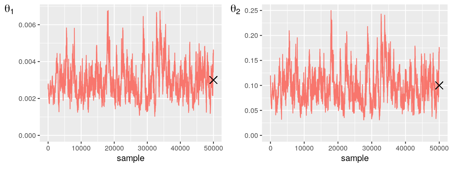
The distribution of samples can also be visualised as a smoothed density or heatmap:
p1 = PlotParameterMarginal(mcmc, 1, tgt)
p2 = PlotParameterHeatmap(mcmc, 1, 2, tgt)
grid.arrange(p1, p2, nrow = 1)
## Don't know how to automatically pick scale for object of type data.frame. Defaulting to continuous.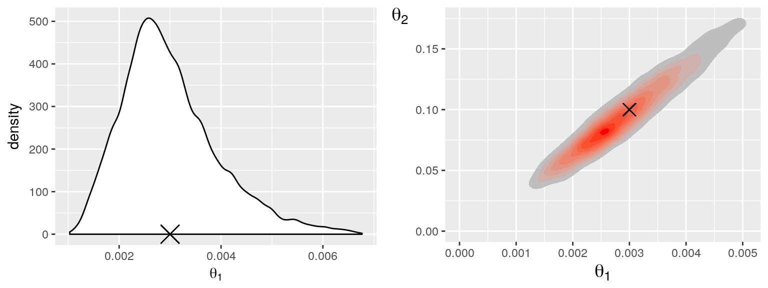
Autocorrelation
Autocorrelation can be used to help determine how well the algorithm mixed by using compute_autocorrelation(rs.mcmc). The autocorrelation function for a single Markov chain is implemented in Discuit using the standard formula:
\(R_l = \frac{\textrm{E} [(X_i - \bar{X})(X_{i+l} - \bar{X})]}{\sigma^2}\)
for any given lag l. The modified formula for multiple chains is given by:
\(R_{b,l} = \frac{\textrm{E} [ (X_i - \bar{X}_b) ( X_{i + l} - \bar{X}_b ) ]}{\sigma^2_b}\)
\(\sigma^2_b = \textrm{E} [(X_i - \bar{X}_b)^2]\)
Autocorrelation can be computed for both single and multiple chains by setting autocorr = TRUE when calling the RunMetHastingsMcmc or RunGelmanDiagnostic functions:
mcmc = RunMetHastingsMcmc(model, y, c(0.0025, 0.12), autocorr = TRUE)
TabulateMcmcSamples(mcmc)
## Theta E(X) SD Mode 95% CI 95% HPD z
## 1 1 0.0032 0.0011 0.0025 (0.0017 - 0.0057) (0.0016 - 0.0053) -0.06
## 2 2 0.11 0.04 0.084 (0.05 - 0.19) (0.046 - 0.19) -0.04Convergence diagnostics
The goal of an MCMC analysis is to construct a Markov chain that has the target distribution as its equilibrium distribution, i.e. it has converged. However assessing whether this is the case can be challenging since we do not know the target distribution. Visual inspection of the Markov chain may not be sufficient to diagnose convergence, particularly where the target distribution has local optima. Automated convergence diagnostics are therefore integrated closely with the MCMC functionality in Discuit; the Geweke test for single chains and the Gelman-Rubin for multiple chains. Just like autocorrelation, the latter, provided that the chains have been initialised with over dispersed parameters (with respect to the target distribution), provides a more reliable indication of algorithm performance (in this case, convergence).
Geweke test of stationarity
The Geweke statistic tests for non-stationarity by comparing the mean and variance for two sections of the Markov chain (see Geweke, 1992; Cowles, 1996). It is given by:
\(z = \frac{\bar{\theta}_{i, \alpha} - \bar{\theta}_{i, \beta}}{\sqrt{Var(\theta_{i, \alpha})+Var(\theta_{i, \beta})})}\)
Geweke statistics are computed automatically for analyses run in Discuit and can be accessed directly (i.e. mcmc$geweke) or else inspected using the PlotGewekeSeries tool, e.g:
PlotGewekeSeries(mcmc)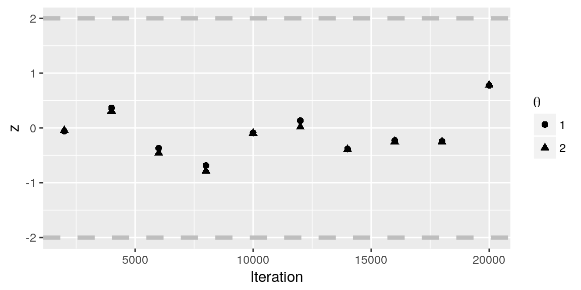
Gelman-Rubin convergence diagnostic
The Gelman-Rubin diagnostic is designed to diagnose convergence of two or more Markov chains by comparing within chain variance to between chain variance (Gelman et al, 1992, 2014). The estimated scale reduction statistic (sometimes referred to as potential scale reduction factor) is calculated for each parameter in the model. Let \(\bar{\theta}\), \(W\) and \(B\) be vectors of length \(P\) representing the mean of model parameters \(\theta\), within chain variance between chain variance respectively for \(M\) Markov chains:
\(W = \frac{1}{M} \sum_{i = 1}^M \sigma^2_i\) \(B = \frac{N}{M - 1} \sum_{i = 1}^M (\hat{\theta}_i - \hat{\theta})^2\)
The estimated scale reduction statistic is given by:
\(R = \sqrt{\frac{d + 3}{d + 1} \frac{N-1}{N} + (\frac{M+1}{MN} \frac{B}{W})}\)
where the first quantity on the RHS adjusts for sampling variance and \(d\) is degrees of freedom estimated using the method of moments.
theta_m = cbind(c(0.0025, 0.003, 0.0035), c(0.12, 0.1, 0.08))
g = RunGelmanDiagnostic(model, y, theta_m)
g$gelman
## parameter mu sre sre_ll sre_ul
## [1,] 1 0.003175533 1.011099 1.002221 1.035468
## [2,] 2 0.105178496 1.004476 1.000868 1.014408For a valid test of convergence the Gelman-Rubin requires two or more Markov chains with over dispersed target values relative to the target distribution. A matrix of such values is therefore required in place of the vector representing the initial values an McMC analysis when calling the function in Discuit, with the \(i^{th}\) row vector used to initialise the \(i^{th}\) Markov chain.
Simulation
The main purpose of the simulation functionality included in Discuit is to provide a source of simulated observations data for evaluation and validation of the MCMC functionality. However simulation can also be an interesting way to explore and better understand the dynamics of the model. To run a simulation and plot the results by using:
x = RunSimulation(model, c(0.003, 0.1), 100.0, 5)
PlotTrajectory(x$trajectory)
## geom_path: Each group consists of only one observation. Do you need to
## adjust the group aesthetic?
Note that the simulation is run for 100.0 time units and 5 observations are drawn. The simulated observations can then be used to validate the model:
mcmc = RunMetHastingsMcmc(model, x$observations, c(0.0025, 0.12))
TabulateMcmcSamples(mcmc)
## Theta E(X) SD Mode 95% CI 95% HPD
## 1 1 7.2e+32 5.5e+32 7.7e+31 (1.6e+31 - 1.7e+33) (4.9e+27 - 1.6e+33)
## 2 2 9.5e+34 6.7e+34 1.2e+34 (7.7e+33 - 2.2e+35) (5.2e+32 - 2.1e+35)
## z
## 1 -1.25
## 2 -1.45