MCMC introduction

Martin Burke

24 August 2018

This article gives a brief introduction to Markov chain Monte Carlo (MCMC) methods and is written for users of the Discuit package who aren’t familiar with MCMC. The article assumes a basic familiarity with Monte Carlo methods, and in particular rejection sampling. See the Monte Carlo introduction article for a basic overview.

The code examples included are written in Python. However users of other languages such as R and Julia should not feel too discouraged since Python is an intuitive language known for its readibility (“runnable pseudocode”). The Jupyter notebook version of this article can be found here.

Introduction to MCMC

The Metropolis-Hastings algorithm

The Metropolis-Hastings algorithm implemented in Discuit is of a class known as ‘random walk’ Markov chain Monte Carlo (MCMC) algorithms. Random walk MCMC algorithms work by ‘exploring’ the parameter space in such a way that the coordinates visited (samples) converge upon the target distribution.

They are another way of obtaining samples from the target distribution \(F\). Like the basic rejection sampler the Metropolis-Hastings draws samples from a proposal distribution and accepts them with a given probability to form a chain.

It is referred to as a Markov chain because each sample depends only on the previous sample. The denominator of the acceptance probability equation is also that of the previous sample \(x_i\).

Example

First we import some things and define a couple of likelihood functions.

# import some stuff for random number generation, analysis and plotting
import numpy as np
import pandas as pd
from plotnine import *
from plotnine.data import *

# likelihood function
def correct_likelihood(z):
    comb = 6 - abs(z - 7)
    return comb * 1/36


# likelihood estimator
def dodgy_likelihood(z):
    like = correct_likelihood(z)
    pert = (np.random.random() - 0.5) * 0.1
    return max(like + pert, 0)

/usr/lib/python3.6/importlib/_bootstrap.py:219: RuntimeWarning: numpy.dtype size changed, may indicate binary incompatibility. Expected 96, got 88
  return f(*args, **kwds)
/usr/lib/python3.6/importlib/_bootstrap.py:219: RuntimeWarning: numpy.dtype size changed, may indicate binary incompatibility. Expected 96, got 88
  return f(*args, **kwds)

In the simple rejection sampler we made proposals independently by drawing a random number between two and twelve. In this example we shall propose the new state \(x_f\) by drawing a random number (which may be positive or negative) and adding it to \(x_i\):

# metropolis hastings algorithm
PROPOSAL = 8    # jump size


def met_hastings_alg(steps, likelihood_function):
    #initialise
    xi = 2
    lik_xi = likelihood_function(xi)
    lik_err = lik_xi - correct_likelihood(xi)
    markov_chain = list()
    num_accept = 0
    # get some samples
    for x in range(1, steps + 1):
        # propose new state
        xf = xi + np.random.randint(-PROPOSAL, PROPOSAL+1)
        # evaluate likelihood
        lik_xf = likelihood_function(xf)
        # accept with mh probability
        accept = False
        mh_prop = lik_xf / lik_xi
        if mh_prop > 1:
            # accept automatically
            accept = True
        else:
            # accept sometimes
            if np.random.random() < mh_prop:
                accept = True
        # add sample to mc
        if accept:
            num_accept = num_accept + 1
        rowi = (x, xi, lik_xi, xf, lik_xf, accept, num_accept / x, lik_err)
        markov_chain.append(rowi)
        # update xi
        if accept:
            xi = xf
            lik_xi = lik_xf
            lik_err = lik_xi - correct_likelihood(xi)
    # create data frame and return
    return pd.DataFrame(markov_chain, columns=["i", "xi", "lik_xi", "xf", "lik_xf", "accept", "ar", "lik_err"])

Now we run can run the algorithm. Usually we would discard a number initial samples to allow the algorithm to ‘converge’ upon the desired distribution but that is not necessary in this example. the al

# run markov chain 
mc = met_hastings_alg(1000, dodgy_likelihood)
p = ggplot(mc, aes(x = "xi", y = "..density..")) + geom_histogram(binwidth=1)
print(p)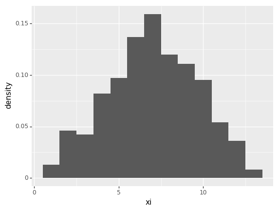

png

<ggplot: (8751541417136)>

We can use a ‘traceplot’ to examine the path of the algorithm:

trace = ggplot(mc, aes(x = "i", y = "xi")) + geom_line()
print(trace)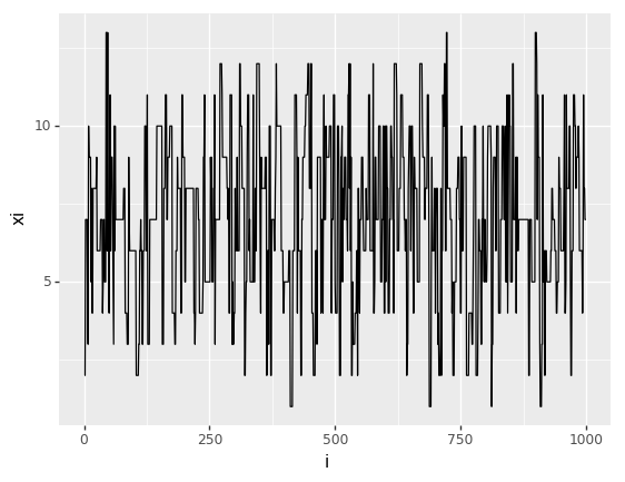

png

<ggplot: (8751541388471)>

Summary

MCMC can be a useful tool for sampling from high dimensional or othertypes of probability distribution that are difficult to sample directly. This is the main rationale for use of the algorithm in the Discuit package. See the package documentation for Discuit.jl (Julia) and Discuit (R) for examples of MCMC in discrete state space continuous time (DSSCT) models.