Discuit.jl models
This section describes the library of predefined models in Discuit. Models can also be user defined, or generated and modified according to need. The models included are mostly epidemiological (see Miscellaneous for other types of model). The next section described the model generating function and an overview of default model components.
Generating models
Pre defined models can be invoked by calling:
generate_model(model_name, initial_condition, σ = 2.0)Examples
model = generate_model("SIS", [100, 1]]);
model = generate_model("SEIR", [100, 0, 1, 0]], 1.0)
Defaults
Discuit.jl models are mutable structs so it is convenient to generate pre defined models with default values for most things and overwrite as required. Only the model_name and initial_condition are required to call generate_model. The following gives an overview of important defaults that the user should note before proceeding with their analysis.
Observation function
The default model.obs_function returns a vector representing the state of the system at obsertion time $t_y$, i.e.:
obs_fn(population::Array{Int64, 1}) = populationObservation likelihood model
The default model.observation_model is Gaussian with observation error σ = 2.0 by default, which can be changed by providing an optional third parameter to generate_model per the example above,
ADD latex.
Prior density function
The default model.prior density function is weak, e.g. in a simple two parameter model it is equivalent to:
function weak_prior(parameters::Array{Float64, 1})
    parameters[1] > 0.0 || return 0.0
    parameters[2] > 0.0 || return 0.0
    return 1.0
end
Note that all models generated by the ADD XREF have t0_index = 0 by default and that changing this parameter will likely require replacing the the density with something like:
function weak_prior(parameters::Array{Float64, 1})
    parameters[1] > 0.0 || return 0.0
    parameters[2] > 0.0 || return 0.0
    parameters[3] < 0.0 || return 0.0
    return 1.0
end
where parameters[3] is designated as the, e.g. initial infection, which is assumed to have taken place prior to e.g. the initial observation at t = 0.0.
Standard Kermack-McKendrick models
The standard Kermack-McKendrick SIR model can be used to model diseases which confer lasting immunity or situations where infected individuals have been detected and quarantined for treatment (Kermack and McKendrick, 1991). ADD REF: kermackcontributions1991
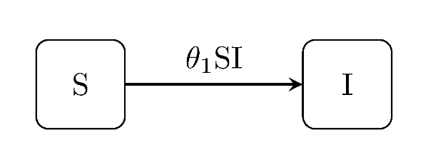
Discuit.generate_model("SI", [100, 1])The susceptible-infectious ("SI") is a very basic model with only one type of event. Individuals who become infected remain infected for the duration of trajectory:
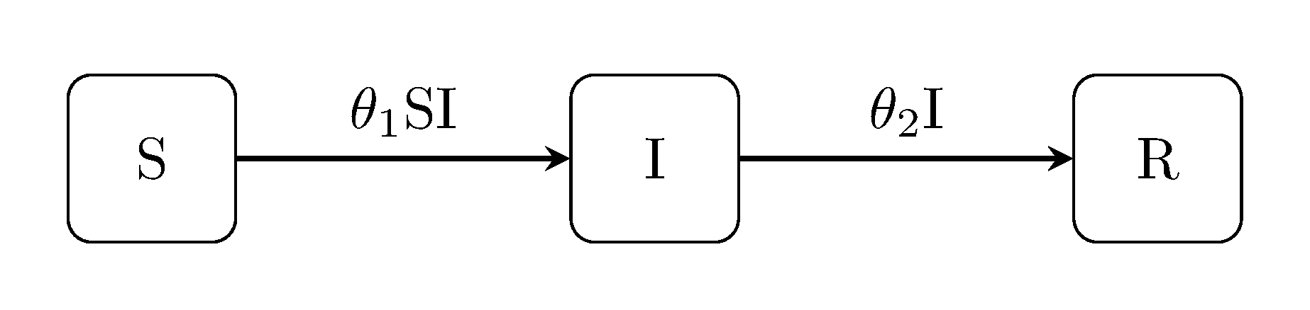
Discuit.generate_model("SIR", [100, 1, 0])The classic Kermack-McKendrick susceptible-infectious-recovered ("SIR") model includes an extra 'recovery' event and an additional compartment for recovered individuals:
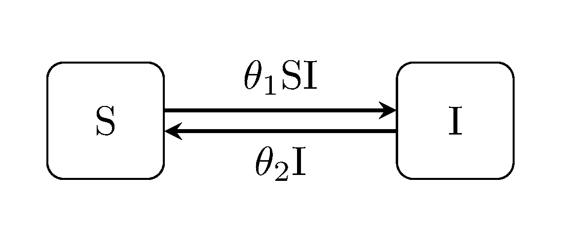
Discuit.generate_model("SIS", [100, 1])The susceptible-infectious-susceptible ("SIS") model is an extension of the classic Kermack-McKendrick SIR model for diseases which do not confer lasting immunity:

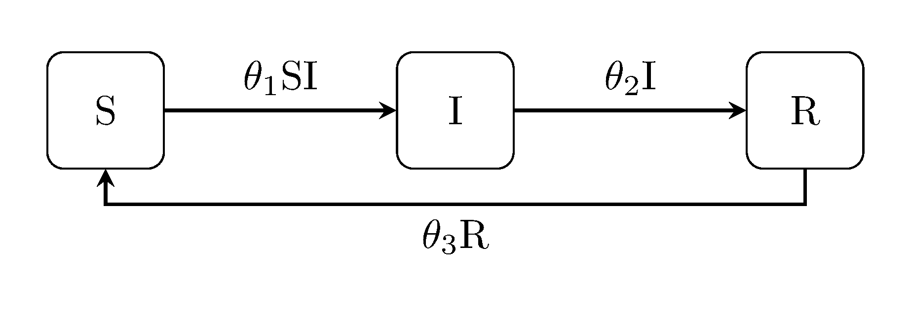
Discuit.generate_model("SIRS", [100, 1, 0])The susceptible-infectious-recovered-susceptible ("SIRS") model incorporates all of the above, i.e. it is for diseases which do not confer long lasting immunity.
Latent Kermack-McKendrick models
The next class of models extend the classic Kermack-McKendrick by accounting for an exposed state E between infection and the onset of infectiousness. For example, the susceptible-exposed-infectious SEI model:
Discuit.generate_model("SEI", [100, 1, 0])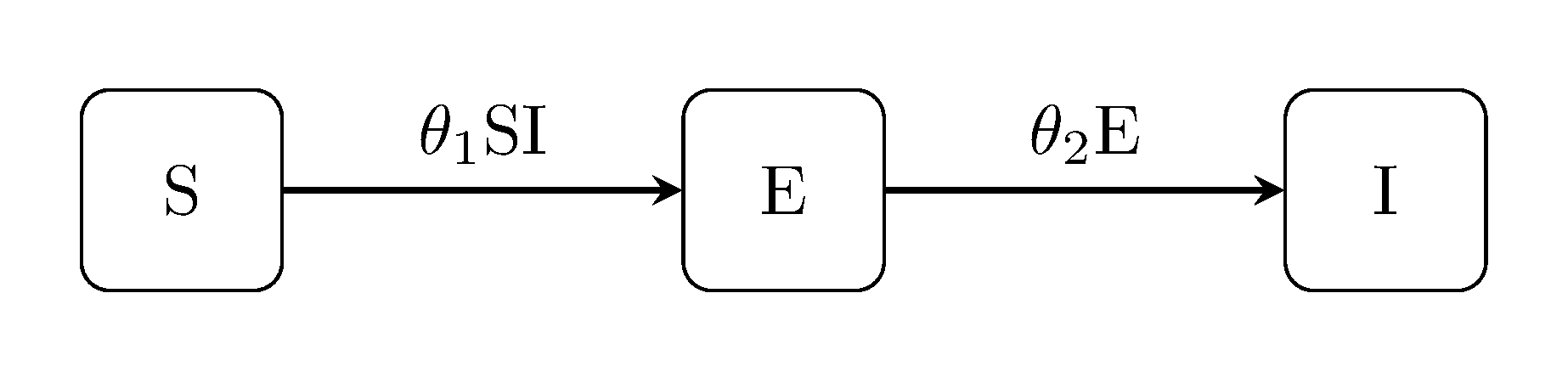
The latent Kermack-McKendrick models can be extended in the same way, i.e, the SEIR model, SEIS and SEIRS:
Discuit.generate_model("SEIR", [100, 1, 0, 0])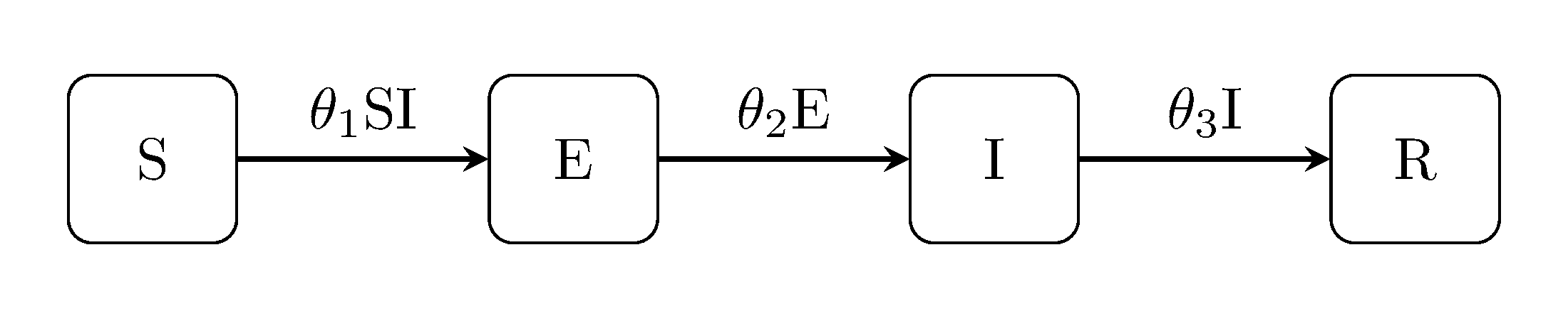
Discuit.generate_model("SEIS", [100, 1, 0])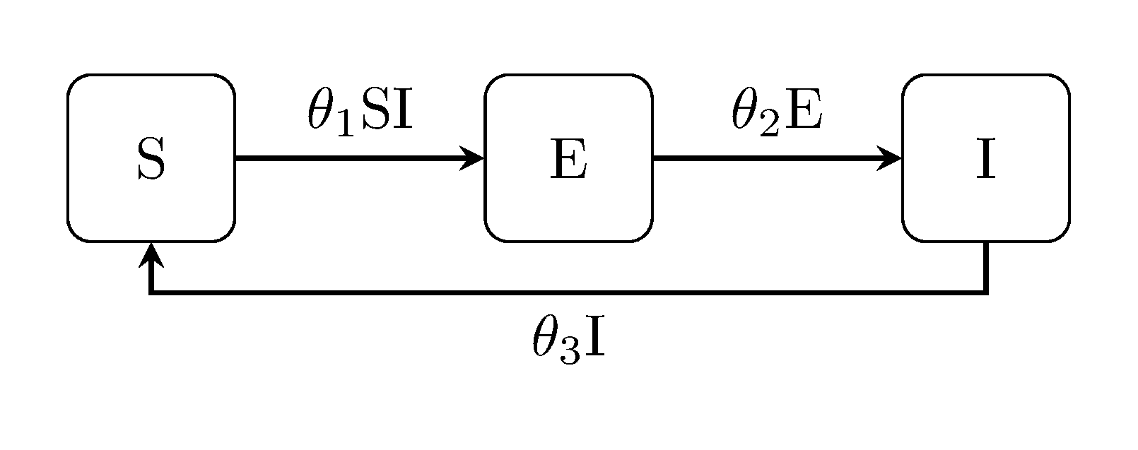
Discuit.generate_model("SEIRS", [100, 1, 0, 0])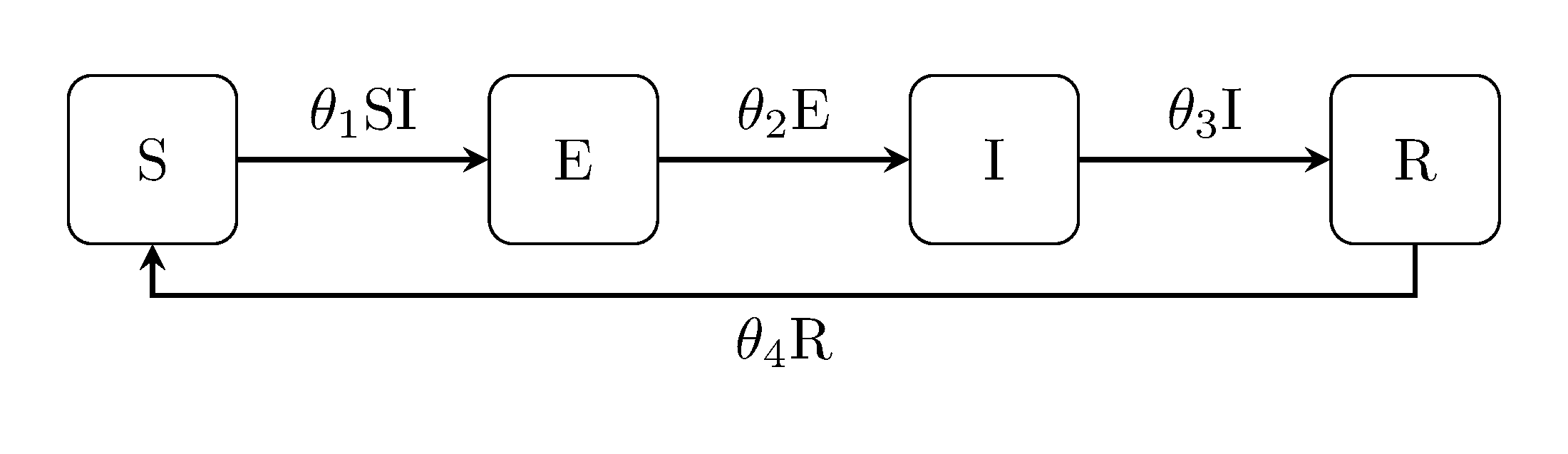
Miscellaneous
Lotka-Volterra predator-prey model
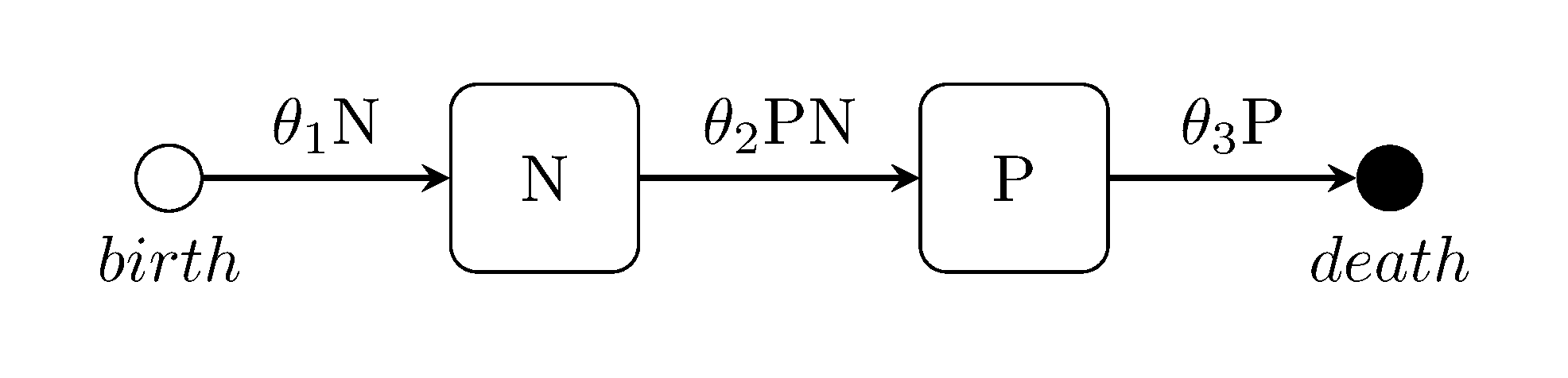
The Lotka-Volterra model is well known for its application to predator-prey interactions but can also be used to model chemical, bio molecular and other auto regulating biological systems. Compartments are labelled Predator, pRey. The model.rate_function for prey reproduction, predator reproduction and predator death is defined as:
function lotka_rf(output, parameters::Array{Float64, 1}, population::Array{Int64, 1})
  # prey; predator reproduction; predator death
  output[1] = parameters[1] * population[2]
  output[2] = parameters[2] * population[1] * population[2]
  output[3] = parameters[3] * population[1]
end
with the transition matrix given as:
m_transition = [ 0 1; 1 -1; -1 0 ]Ross-MacDonald malaria model
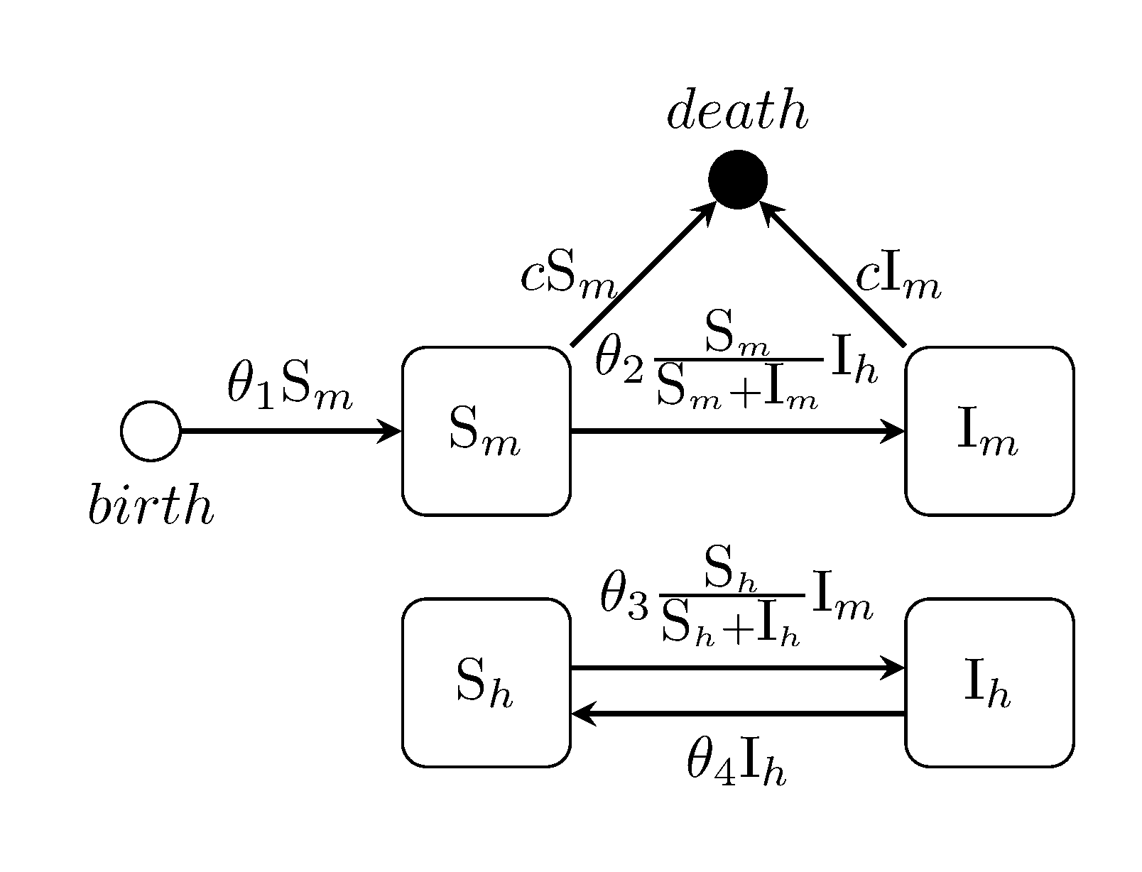
The Ross-MacDonald malaria model is an extension of the Kermack-McKendrick SIS model which accounts for two species, human and mosquito. ADD CITATION. This example is simplified in two ways...
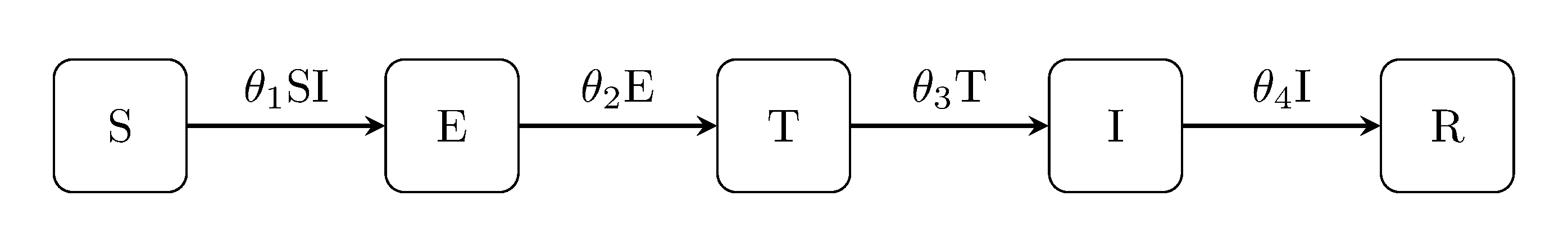
SETIR model for bTB
More information
ADD list...
[Compartmental models in epidemiology](https://en.wikipedia.org/wiki/Compartmentalmodelsin_epidemiology] (Wiki).
References