Discuit.jl examples
The following examples provide a flavour of package's core functionality. See the Discuit.jl manual for a description of the data types and functions in Discuit, and Discuit.jl models for a description of the predefined models available in the package. The tutorial is designed to be run using the REPL but usually it is wise to save code and analyses to a text file for reference later. By convention Julia code files have the extension '.jl'. For example, the file pooley_model.jl (click to download) contains code equivalent to the next section, i.e. it defines a SIS model and stores it in variable model which can then be used just as if we had typed the commands manually.
One way to run a code file is to open a command prompt or terminal and cd to the location of the file. Check the code and save the file. Next start the REPL using the command julia. Finally type the name of the file to run the code:
ADD GIF
Defining a model
DiscuitModels can be created automatically using helper functions or manually by specifying each component. For example the model we are about to create could be generated automatically using generate_model("SIS", [100,1]). However constructing it manually is a helpful exercise for getting to know the package. See Discuit.jl models for further details of the generate_model function. We start by examining DiscuitModel in the package documentation:
julia> using Discuit;The events in a DiscuitModel are defined by the rates at which they occur and a transition matrix, which governs how individuals migrate between states. In the basic Kermack-McKendrick SIS (and SIR) model, rates for infection and recovery events respectively are given by:
With the transition matrix:
Note how the first row of the matrix reflects the removal of a susceptible individual from the S state, and migrates them to the second element of the row, the 'I' state. The code required to represent the rates (or 'rate function') and transition matrxi as Julia variables is correspondingly straightforward:
julia> function sis_rf(output::Array{Float64, 1}, parameters::Array{Float64, 1}, population::Array{Int64, 1})
           output[1] = parameters[1] * population[1] * population[2]
           output[2] = parameters[2] * population[2]
       end
sis_rf (generic function with 1 method)

julia> t_matrix = [-1 1; 1 -1]
2×2 Array{Int64,2}:
 -1   1
  1  -1
The output confirms that sis_rf, a generic function with 1 method has been defined and gives a description of the 2 dimensional Array variable that represents the transition matrix (do not copy and paste these bits when running the code on your own machine). Note that the correct function signature must be used in the implementation for it to be compatible with the package. In this case the function takes three Array parameters of a given type, the first of which is the output variable modified by the function (which is why it does not need to return any actual output variable). Next we define a simple observation function, again with the correct signature:
julia> obs_fn(population::Array{Int64, 1}) = population
obs_fn (generic function with 1 method)
The default prior distribution is flat and improper, and is equivalent to:
julia> function weak_prior(parameters::Array{Float64, 1})
           parameters[1] > 0.0 || return 0.0
           parameters[2] > 0.0 || return 0.0
           return 1.0
       end
weak_prior (generic function with 1 method)
Finally, we define an observation likelihood model. Again, we use the same as Pooley, with observation errors normally distributed around the true value with standard deviation 2:
julia> function si_gaussian(y::Array{Int64, 1}, population::Array{Int64, 1})
           obs_err = 2
           tmp1 = log(1 / (sqrt(2 * pi) * obs_err))
           tmp2 = 2 * obs_err * obs_err
           obs_diff = y[2] - population[2]
           return tmp1 - ((obs_diff * obs_diff) / tmp2)
       end
si_gaussian (generic function with 1 method)
We can now define a model. We must also specify the initial_condition which represents the state of the population at the origin of each trajectory. A final parameter declared inline is an optional index for the t0 parameter (ignore for now):
julia> initial_condition = [100, 1]
2-element Array{Int64,1}:
 100
   1

julia> model = DiscuitModel("SIS", initial_condition, sis_rf, t_matrix, obs_fn, weak_prior, si_gaussian, 0);
MCMC
The following example is based on that published by Pooley et al. (2015) in the paper that introduces the model based proposal method. The observations data simulated by Pooley can be downloaded here and saved, e.g. to path/to/data/. Next, load the observations data using:
y = get_observations("path/to/data/pooley.csv")Now we can run an MCMC analysis based on the simulated datset:
julia> rs = run_met_hastings_mcmc(model, y, [0.0025, 0.12]);
running MCMC...
 finished (sample μ = [0.0034241420925407253, 0.11487898025205769])
Visual inspection of the Markov chain using the traceplot is one way of assessing the convergence of the algorithm:
julia> plot_parameter_trace(rs, 1)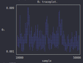
The marginal distribution of parameters can be plotted by calling:
julia> plot_parameter_marginal(rs, 1)
┌ Warning: The keyword parameter `bins` is deprecated, use `nbins` instead
│   caller = ip:0x0
└ @ Core :-1
                       ┌                                        ┐
      [0.001 , 0.0015) ┤▇ 295
      [0.0015, 0.002 ) ┤▇▇▇▇▇▇▇▇▇▇▇▇▇▇▇ 3378
      [0.002 , 0.0025) ┤▇▇▇▇▇▇▇▇▇▇▇▇▇▇▇▇▇▇▇▇▇▇▇▇▇▇▇▇▇▇▇ 6960
      [0.0025, 0.003 ) ┤▇▇▇▇▇▇▇▇▇▇▇▇▇▇▇▇▇▇▇▇▇▇▇▇▇▇▇▇▇▇▇▇▇▇ 7700
      [0.003 , 0.0035) ┤▇▇▇▇▇▇▇▇▇▇▇▇▇▇▇▇▇▇▇▇▇▇▇▇▇▇▇▇▇▇▇▇ 7265
      [0.0035, 0.004 ) ┤▇▇▇▇▇▇▇▇▇▇▇▇▇▇▇▇▇▇▇▇▇▇▇▇ 5425
      [0.004 , 0.0045) ┤▇▇▇▇▇▇▇▇▇▇▇▇▇▇ 3148
      [0.0045, 0.005 ) ┤▇▇▇▇▇▇▇▇▇ 2092
      [0.005 , 0.0055) ┤▇▇▇▇▇ 1023
      [0.0055, 0.006 ) ┤▇▇▇ 675
      [0.006 , 0.0065) ┤▇▇ 494
   θ₁ [0.0065, 0.007 ) ┤▇ 271
      [0.007 , 0.0075) ┤ 68
      [0.0075, 0.008 ) ┤▇ 138
      [0.008 , 0.0085) ┤ 76
      [0.0085, 0.009 ) ┤ 80
      [0.009 , 0.0095) ┤ 111
      [0.0095, 0.01  ) ┤▇ 273
      [0.01  , 0.0105) ┤▇ 195
      [0.0105, 0.011 ) ┤▇ 133
      [0.011 , 0.0115) ┤ 67
      [0.0115, 0.012 ) ┤ 77
      [0.012 , 0.0125) ┤ 57
                       └                                        ┘
                                        samples
Plotting the data with third party packages such as PyPlot is simple:
using PyPlot
x = mcmc.samples[mcmc.adapt_period:size(mcmc.samples, 1), parameter]
plt[:hist](x, 30)
xlabel(string("\$\\theta_", parameter, "\\$"))
ylabel("density")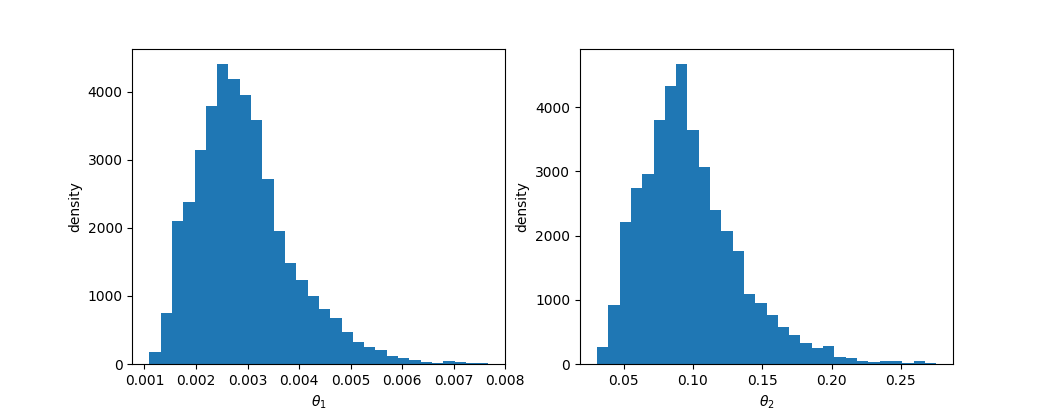
A pairwise representation can be produced by calling plot_parameter_heatmap (see below for an example).
Autocorrelation
Autocorrelation can be used to help determine how well the algorithm mixed by using compute_autocorrelation. The autocorrelation function for a single Markov chain is implemented in Discuit using the standard formula:
for any given lag l. The modified formula for multiple chains is given by:
julia> ac = compute_autocorrelation(rs);

julia> plot_autocorrelation(ac)
                   θ autocorrelation
       ┌────────────────────────────────────────┐
     1 │⢧⠀⠀⠀⠀⠀⠀⠀⠀⠀⠀⠀⠀⠀⠀⠀⠀⠀⠀⠀⠀⠀⠀⠀⠀⠀⠀⠀⠀⠀⠀⠀⠀⠀⠀⠀⠀⠀⠀⠀│
       │⠈⣧⠀⠀⠀⠀⠀⠀⠀⠀⠀⠀⠀⠀⠀⠀⠀⠀⠀⠀⠀⠀⠀⠀⠀⠀⠀⠀⠀⠀⠀⠀⠀⠀⠀⠀⠀⠀⠀⠀│
       │⠀⠘⣧⠀⠀⠀⠀⠀⠀⠀⠀⠀⠀⠀⠀⠀⠀⠀⠀⠀⠀⠀⠀⠀⠀⠀⠀⠀⠀⠀⠀⠀⠀⠀⠀⠀⠀⠀⠀⠀│
       │⠀⠀⠙⡷⡄⠀⠀⠀⠀⠀⠀⠀⠀⠀⠀⠀⠀⠀⠀⠀⠀⠀⠀⠀⠀⠀⠀⠀⠀⠀⠀⠀⠀⠀⠀⠀⠀⠀⠀⠀│
       │⠀⠀⠀⠘⢎⠢⡀⠀⠀⠀⠀⠀⠀⠀⠀⠀⠀⠀⠀⠀⠀⠀⠀⠀⠀⠀⠀⠀⠀⠀⠀⠀⠀⠀⠀⠀⠀⠀⠀⠀│
       │⠀⠀⠀⠀⠀⠑⣍⢦⡀⠀⠀⠀⠀⠀⠀⠀⠀⠀⠀⠀⠀⠀⠀⠀⠀⠀⠀⠀⠀⠀⠀⠀⠀⠀⠀⠀⠀⠀⠀⠀│
       │⠀⠀⠀⠀⠀⠀⠈⠳⣝⠦⡀⠀⠀⠀⠀⠀⠀⠀⠀⠀⠀⠀⠀⠀⠀⠀⠀⠀⠀⠀⠀⠀⠀⠀⠀⠀⠀⠀⠀⠀│
   R   │⠀⠀⠀⠀⠀⠀⠀⠀⠀⠑⠮⣗⣤⡀⠀⠀⠀⠀⠀⠀⠀⠀⠀⠀⠀⠀⠀⠀⠀⠀⠀⠀⠀⠀⠀⠀⠀⠀⠀⠀│
       │⠀⠀⠀⠀⠀⠀⠀⠀⠀⠀⠀⠀⠉⠛⢗⣄⠀⠀⠀⠀⠀⠀⠀⠀⠀⠀⠀⠀⠀⠀⠀⠀⠀⠀⠀⠀⠀⠀⠀⠀│
       │⠀⠀⠀⠀⠀⠀⠀⠀⠀⠀⠀⠀⠀⠀⠀⠑⢗⣄⠀⠀⠀⠀⠀⠀⠀⠀⠀⠀⠀⠀⠀⠀⠀⠀⠀⠀⠀⠀⠀⠀│
       │⠀⠀⠀⠀⠀⠀⠀⠀⠀⠀⠀⠀⠀⠀⠀⠀⠀⠙⣧⡀⠀⠀⠀⠀⠀⠀⠀⠀⠀⠀⠀⠀⠀⠀⠀⠀⠀⠀⠀⠀│
       │⠀⠀⠀⠀⠀⠀⠀⠀⠀⠀⠀⠀⠀⠀⠀⠀⠀⠀⠈⠻⡦⣄⠀⠀⠀⠀⠀⠀⠀⠀⠀⠀⠀⠀⠀⠀⠀⠀⠀⠀│
       │⠀⠀⠀⠀⠀⠀⠀⠀⠀⠀⠀⠀⠀⠀⠀⠀⠀⠀⠀⠀⠈⠛⢗⡦⣄⣀⠀⠀⠀⠀⠀⠀⠀⠀⠀⠀⠀⠀⠀⠀│
       │⠀⠀⠀⠀⠀⠀⠀⠀⠀⠀⠀⠀⠀⠀⠀⠀⠀⠀⠀⠀⠀⠀⠀⠈⠉⠙⠛⠳⠶⢦⣤⣄⡀⠀⠀⠀⠀⠀⠀⠀│
     0 │⠀⠀⠀⠀⠀⠀⠀⠀⠀⠀⠀⠀⠀⠀⠀⠀⠀⠀⠀⠀⠀⠀⠀⠀⠀⠀⠀⠀⠀⠀⠀⠉⠛⢷⣦⣀⣀⣀⣀⣀│
       └────────────────────────────────────────┘
       0                                     2000
                          lag
Note that the latter formulation (for multiple chains) is likely to give a more accurate indication of algorithm performance. The code is virtually identical. Just replace rs with the results of a call to run_gelman_diagnostic.
Convergence diagnostics
The goal of an MCMC analysis is to construct a Markov chain that has the target distribution as its equilibrium distribution, i.e. it has converged. However assessing whether this is the case can be challenging since we do not know the target distribution. Visual inspection of the Markov chain may not be sufficient to diagnose convergence, particularly where the target distribution has local optima. Automated convergence diagnostics are therefore integrated closely with the MCMC functionality in Discuit; the Geweke test for single chains and the Gelman-Rubin for multiple chains. Just like autocorrelation, the latter, provided that the chains have been initialised with over dispersed parameters (with respect to the target distribution), provides a more reliable indication of algorithm performance (in this case, convergence).
Geweke test of stationarity
The Geweke statistic tests for non-stationarity by comparing the mean and variance for two sections of the Markov chain (see Geweke, 1992; Cowles, 1996). It is given by:
Geweke statistics are computed automatically for analyses run in Discuit and can be accessed directly (i.e. rs.geweke) or else inspected using one of the built in tools, e.g:
julia> plot_geweke_series(rs)
        ┌────────────────────────────────────────┐
      2 │⠉⠉⠉⠉⠉⠉⠉⠉⠉⠉⠉⠉⠉⠉⠉⠉⠉⠉⠉⠉⠉⠉⠉⠉⠉⠉⠉⠉⠉⠉⠉⠉⠉⠉⠉⠉⠉⠉⠉⠉│
        │⠀⠀⠀⠀⠀⠀⠀⠀⠀⠀⠀⠀⠀⠀⠀⠀⠀⠀⠀⠀⠀⠀⠀⠀⠀⠀⠀⠀⠀⠀⠀⠀⠀⠀⠀⠀⠀⠀⠀⠀│
        │⠀⠀⠀⠀⠀⠀⠀⠀⠀⠀⠀⠀⠀⠀⠀⠀⠀⠀⠀⠀⠀⠀⠀⠀⠀⠀⠀⠀⠀⠀⠀⠀⠀⠀⠀⠀⠀⠀⠀⠀│
        │⠀⠀⠀⠀⠀⠀⠀⠀⠀⠀⠀⠀⠀⠀⠀⠀⠀⠀⠀⠀⠀⠀⠀⠀⠀⠀⠀⠀⠀⠀⠀⠀⠆⠀⠀⠀⠀⠀⠀⠀│
        │⠀⠀⠀⠀⠀⠀⠀⠀⠀⠀⠀⠀⠀⠀⠀⠀⠀⠀⠀⠀⠀⠀⠀⠀⠀⠀⠀⠀⠀⠀⠀⠀⠀⠀⠀⠀⠀⠀⠀⠀│
        │⠀⠀⠀⠀⠀⠀⠀⠀⠀⠀⠀⠀⠀⠀⠀⠀⠀⠀⠀⠀⠀⠀⠀⠀⠀⠀⠀⠀⠀⠀⠀⠀⠀⠀⠀⠀⠀⠀⠀⠀│
        │⠀⠀⠀⠀⠀⠀⠀⠀⠀⠀⠀⠀⠀⠀⠀⠀⠀⠀⠀⠀⠀⠀⠀⠀⠀⠀⠀⠀⠀⠀⠀⠀⠀⠀⠀⠀⠀⠀⠀⠀│
   z    │⠀⠀⠀⠀⠀⠀⠀⠀⠀⠀⠀⠀⠀⠀⠀⠀⠀⠀⠀⠀⠀⠀⠀⠀⠀⠀⠀⠀⠀⠀⠀⠀⠀⠀⠀⠀⠀⠀⠀⠀│
        │⠀⠀⠀⠀⠀⠀⠀⠀⠀⠀⠀⠀⠀⠀⠀⠀⠀⠀⠀⠀⠀⠀⠀⠀⠀⠀⠀⠀⠀⠀⠀⠀⠀⠀⠀⠀⠀⠀⠀⠀│
        │⠀⠀⠀⠀⠀⠀⠀⠀⠀⠀⠀⠀⠀⠀⠀⠀⠀⠀⠀⠀⠀⠀⠀⠀⠀⠀⠀⠀⠀⠀⠀⠀⠀⠀⠀⠀⠀⠀⠀⠀│
        │⠉⠉⠉⠉⡉⠉⠉⠉⡍⠉⠉⠉⠉⠉⠉⠉⠉⠉⠉⠉⠋⠉⠉⠉⠉⠉⠉⠉⡍⠉⠉⠉⠉⠉⠉⠉⠉⠉⠉⠉│
        │⠀⠀⠀⠀⠁⠀⠀⠀⠀⠀⠀⠀⠄⠀⠀⠀⠀⠀⠀⠀⠀⠀⠀⠀⠀⠀⠀⠀⠀⠀⠀⠀⠀⠀⠀⠀⠁⠀⠀⠀│
        │⠀⠀⠀⠀⠀⠀⠀⠀⠀⠀⠀⠀⠀⠀⠀⠀⠄⠀⠀⠀⠀⠀⠀⠀⠄⠀⠀⠀⠀⠀⠀⠀⠀⠀⠀⠀⠀⠀⠀⠘│
        │⠀⠀⠀⠀⠀⠀⠀⠀⠀⠀⠀⠀⠀⠀⠀⠀⠀⠀⠀⠀⠀⠀⠀⠀⠀⠀⠀⠀⠀⠀⠀⠀⠀⠀⠀⠀⠀⠀⠀⠀│
     -1 │⠀⠀⠀⠀⠀⠀⠀⠀⠀⠀⠀⠀⠀⠀⠀⠀⠀⠀⠀⠀⠀⠀⠀⠀⠀⠀⠀⠀⠀⠀⠀⠀⠀⠀⠀⠀⠀⠀⠀⠀│
        └────────────────────────────────────────┘
        0                                    20000
Note that the results of MCMC analyses, including Geweke statistics, can be saved to file for analysis in the companion R package. In Julia, run:
print_mcmc_results(rs, "path/to/mcmc/data/")Now, in R, run:
library(Discuit)
library(gridExtra)
rs = LoadMcmcResults("path/to/mcmc/data/")
tgt = c(0.003, 0.1)
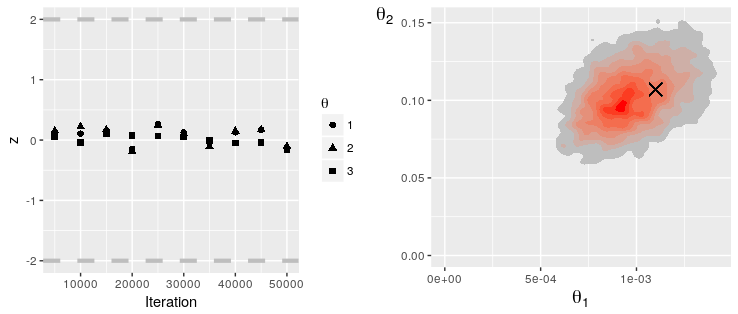
grid.arrange(PlotGewekeSeries(rs), PlotParameterHeatmap(rs, 1, 2, tgt), nrow = 1)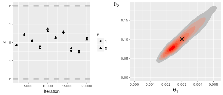
Gelman-Rubin convergence diagnostic
The Gelman-Rubin diagnostic is designed to diagnose convergence of two or more Markov chains by comparing within chain variance to between chain variance (Gelman et al, 1992, 2014). The estimated scale reduction statistic (sometimes referred to as potential scale reduction factor) is calculated for each parameter in the model.
Let $\bar{\theta}$, $W$ and $B$ be vectors of length $P$ representing the mean of model parameters $\theta$, within chain variance between chain variance respectively for $M$ Markov chains:
The estimated scale reduction statistic is given by:
where the first quantity on the RHS adjusts for sampling variance and $d$ is degrees of freedom estimated using the method of moments. For a valid test of convergence the Gelman-Rubin requires two or more Markov chains with over dispersed target values relative to the target distribution. A matrix of such values is therefore required in place of the vector representing the initial values an McMC analysis when calling the function in Discuit, with the $i^{th}$ row vector used to initialise the $i^{th}$ Markov chain.
julia> rs = run_gelman_diagnostic(model, y, [0.0025 0.08; 0.003 0.12; 0.0035 0.1]);
running gelman diagnostic... (3 chains)
 chain 1 complete on thread 1
 chain 2 complete on thread 1
 chain 3 complete on thread 1
 finished (sample μ = [0.00305, 0.101]).
Simulation
The main purpose of the simulation functionality included in Discuit is to provide a source of simulated observations data for evaluation and validation of the MCMC functionality. However simulation can also be an interesting way to explore and better understand the dynamics of the model.
To produce the Lotka-Volterra example given in the paper use:
julia> model = generate_model("LOTKA", [79, 71]);

julia> xi = gillespie_sim(model, [0.5, 0.0025, 0.3]);
running simulation...
 finished (17520 events).

julia> plot_trajectory(xi)
                                PN simulation
                  ┌────────────────────────────────────────┐
              500 │⠀⠀⠀⠀⠀⠀⠀⠀⠀⠀⠀⠀⠀⠀⠀⠀⠀⠀⠀⠀⠀⠀⠀⠀⠀⠀⠀⠀⠀⠀⠀⠀⠀⠀⠀⠀⠀⠀⠀⠀│ P
                  │⠀⠀⠀⠀⠀⠀⠀⠀⠀⠀⠀⠀⠀⠀⠀⠀⠀⠀⠀⠀⠀⠀⠀⠀⠀⠀⠀⠀⠀⠀⠀⠀⠀⠀⠀⠀⠀⠀⠀⠀│ N
                  │⠀⠀⠀⡄⠀⠀⠀⠀⠀⠀⠀⠀⠀⠀⠀⠀⠀⠀⠀⠀⠀⠀⠀⠀⠀⠀⠀⠀⠀⠀⣠⠀⠀⠀⠀⠀⠀⠀⠀⠀│
                  │⠀⠀⢸⢧⠀⠀⠀⠀⠀⠀⠀⠀⠀⠀⠀⠀⠀⠀⠀⠀⠀⠀⠀⠀⠀⠀⠀⠀⠀⠀⣿⠀⠀⠀⠀⠀⠀⠀⠀⠀│
                  │⠀⠀⢸⢸⠀⠀⠀⠀⠀⠀⠀⠀⠀⠀⠀⠀⠀⠀⠀⠀⠀⠀⠀⠀⠀⠀⠀⠀⠀⠀⣿⡀⠀⠀⠀⠀⠀⠀⠀⠀│
                  │⠀⢀⢸⢸⡀⠀⠀⠀⠀⠀⢰⣇⠀⠀⠀⠀⠀⠀⠀⠀⠀⠀⠀⠀⠀⠀⠀⠀⠀⢠⠇⡇⠀⠀⠀⠀⣷⠀⠀⠀│
                  │⠀⢸⡏⠀⡇⠀⠀⠀⠀⠀⡟⢹⡀⠀⠀⠀⠀⠀⣶⠀⠀⠀⠀⠀⠀⠀⠀⠀⠀⢸⠀⣇⠀⠀⠀⢰⠿⡄⠀⠀│
   population     │⠀⡞⣧⠀⣇⠀⠀⠀⠀⢠⠇⠀⡇⠀⠀⠀⠀⢸⠙⡇⠀⠀⢸⢶⣴⡄⠀⠀⢠⣾⠀⢸⠀⠀⠀⣸⠀⡇⠀⠀│
                  │⠀⡇⣿⠀⢸⠀⠀⠀⠀⣿⡀⠀⢳⠀⠀⠀⢀⡼⠀⢳⠀⠀⡏⠈⠁⢳⠀⠀⢸⣿⡄⠸⡄⠀⣰⣻⠀⢹⠀⠀│
                  │⠀⣇⣿⠀⠈⣧⠀⠀⣸⣻⣧⠀⢸⡄⠀⠀⣸⢧⠀⢸⡄⢠⡇⠀⠀⠘⡇⠀⡞⡇⡇⠀⣇⠀⡏⡏⡇⠈⡇⠀│
                  │⢸⢹⢸⠀⠀⠘⣇⢀⣯⡇⢸⡀⠀⢳⣠⢶⠟⠸⡄⠀⢿⣾⢷⢀⠀⠀⢧⠀⣷⠃⡇⠀⢸⢀⣷⠃⡇⠀⢹⡀│
                  │⢸⢸⠈⡇⠀⠀⠸⣾⠟⠁⠈⣇⠀⠀⢻⡟⠀⠀⢧⠀⢀⡇⠘⠻⣦⠀⠘⢾⡿⠀⢧⠀⠘⣾⡾⠀⢧⠀⠀⢳│
                  │⣏⡞⠀⣇⠀⠀⢀⡟⠀⠀⠀⢹⡀⢰⠋⠀⠀⠀⠘⡆⡾⠀⠀⠀⠸⣆⣴⠏⠀⠀⢸⠀⢀⡿⠃⠀⠸⡄⢀⣰│
                  │⠈⠀⠀⠹⡴⠟⠞⠀⠀⠀⠀⠀⠳⠏⠀⠀⠀⠀⠀⠛⠃⠀⠀⠀⠀⠈⠁⠀⠀⠀⠈⢧⡟⠀⠀⠀⠀⠳⠞⠁│
                0 │⠀⠀⠀⠀⠀⠀⠀⠀⠀⠀⠀⠀⠀⠀⠀⠀⠀⠀⠀⠀⠀⠀⠀⠀⠀⠀⠀⠀⠀⠀⠀⠀⠀⠀⠀⠀⠀⠀⠀⠀│
                  └────────────────────────────────────────┘
                  0                                      100
                                    time
The maximum time of the simulation and number of observations to draw can also be specified, e.g. generate_model("LOTKA", [79, 71], 100.0, 10).
Custom MCMC
In addition to the two proposal algorithms included with the packages by default, Discuit allows for users to develop their own algorithms for data augmented MCMC via the alternative custom MCMC framework, while still taking advantage of features including automated, finite adaptive multivariate θ proposals.
In some cases may wish to simply tweak the proposal algorithms included in the source code repositories for minor performance gains in certain models, but the custom MCMC framework can also be useful in cases where the augmented data aspects of the model have specific or complex constraints, such as the next example which is based on an analysis of a smallpox outbreak within a closed community in Abakaliki, Nigeria by O'Neill and Roberts (ADD CITATION). First we generate a standard SIR model and set the t0_index = 3:
julia> model = generate_model("SIR", [119, 1, 0]);

julia> model.t0_index = 3;
Next we define the "medium" prior used by O'Neill and Roberts, with some help from the Distributions.jl package:
Updating registry at `~/.julia/registries/General`
Updating git-repo `https://github.com/JuliaRegistries/General.git`
[?25l[2K[?25h Resolving package versions...
Installed StatsBase ───── v0.30.0
Installed Distributions ─ v0.20.0
Updating `~/build/mjb3/Discuit.jl/docs/Project.toml`
[31c24e10] + Distributions v0.20.0
Updating `~/build/mjb3/Discuit.jl/docs/Manifest.toml`
[31c24e10] ↑ Distributions v0.19.2 ⇒ v0.20.0
[2913bbd2] ↓ StatsBase v0.31.0 ⇒ v0.30.0
julia> using Distributions;
julia> p1 = Gamma(10, 0.0001);
julia> p2 = Gamma(10, 0.01);
julia> function prior_density(parameters::Array{Float64, 1})
return parameters[3] < 0.0 ? pdf(p1, parameters[1]) * pdf(p2, parameters[2]) * (0.1 * exp(0.1 * parameters[3])) : 0.0
end
prior_density (generic function with 1 method)
julia> model.prior_density = prior_density;The observation model is replaced with one that returns log(1) since we will only propose sequences consitent with the observed recoveries and $\pi(\xi | \theta)$ is evaluated automatically by Discuit):
julia> observation_model(y::Array{Int, 1}, population::Array{Int, 1}) = 0.0
observation_model (generic function with 1 method)

julia> model.observation_model = observation_model;
Next we define an array t to contain the recovery times reported by O'Neill and Roberts and a simple Observations variable which consists of the maximum event time and an empty two dimensional array:
julia> t = [0.0, 13.0, 20.0, 22.0, 25.0, 25.0, 25.0, 26.0, 30.0, 35.0, 38.0, 40.0, 40.0, 42.0, 42.0, 47.0, 50.0, 51.0, 55.0, 55.0, 56.0, 57.0, 58.0, 60.0, 60.0, 61.0, 66.0];

julia> y = Observations([67.0], Array{Int64, 2}(undef, 1, 1))
Observations([67.0], [139627917258272])
We also need to define an initial state using the generate_custom_x0 function using some parameter values and a vector of event times and corresponding event types, consistent with t:
julia> evt_tm = Float64[];

julia> evt_tp = Int64[];

julia> for i in 1:(length(t) - 1)# infections at arbitrary t > t0
           push!(evt_tm, -4.0)
           push!(evt_tp, 1)
       end

julia> for i in eachindex(t)     # recoveries
           push!(evt_tm, t[i])
           push!(evt_tp, 2)
       end

julia> x0 = generate_custom_x0(model, y, [0.001, 0.1, -4.0], evt_tm, evt_tp);
The final step before we run our analysis is to define the algorithm which will propose changes to augmented data (parameter proposals are automatically configured by Discuit). Since it is assumed that the total number of events is known we can construct an algorithm that simply changes the time of an event in the trajectory. Events are chosen and new times drawn from uniform distributions ensuring that:
such that the terms cancel in the Metropolis-Hastings acceptance equation. Some additional information is available regarding the times of recoveries; they are known to within a day. We therefore propose new recovery event times such that they remain within the time frame of a single time unit, which correspond to days in this model:
julia> function custom_proposal(model::PrivateDiscuitModel, xi::MarkovState, xf_parameters::ParameterProposal)
           t0 = xf_parameters.value[model.t0_index]
           ## move
           seq_f = deepcopy(xi.trajectory)
           # choose event and define new one
           evt_i = rand(1:length(xi.trajectory.time))
           evt_tm = xi.trajectory.event_type[evt_i] == 1 ? (rand() * (model.obs_data.time[end] - t0)) + t0 : floor(xi.trajectory.time[evt_i]) + rand()
           evt_tp = xi.trajectory.event_type[evt_i]
           # remove old one
           splice!(seq_f.time, evt_i)
           splice!(seq_f.event_type, evt_i)
           # add new one
           if evt_tm > seq_f.time[end]
               push!(seq_f.time, evt_tm)
               push!(seq_f.event_type, evt_tp)
           else
               for i in eachindex(seq_f.time)
                   if seq_f.time[i] > evt_tm
                       insert!(seq_f.time, i, evt_tm)
                       insert!(seq_f.event_type, i, evt_tp)
                       break
                   end
               end
           end
           # compute ln g(x)
           prop_lk = 1.0
           ## evaluate full likelihood for trajectory proposal and return
           return MarkovState(xi.parameters, seq_f, compute_full_log_like(model, xi.parameters.value, seq_f), prop_lk, 3)
       end # end of std proposal function
custom_proposal (generic function with 1 method)
We can now run the MCMC analysis:
julia> rs = run_custom_mcmc(model, y, custom_proposal, x0, 120000, 20000);
running custom MCMC...
ERROR: UndefVarError: compute_full_log_like not defined
The output from the custom MCMC functionality is in the same format as the those produced using the core functions and thus be analysed in the same way. In this case the results were saved to file and analysed in R, in the manner described above:
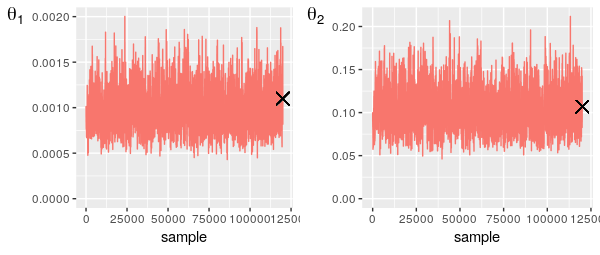
The traceplots indicate good mixing and the results are fairly similar to that obtained by O'Neill and Roberts given the differences in the models used.
References