Simple example

Introduction

Here we introduce the main features of the package using a simple example based on the one in the paper published by Pooley et al that described the model-based-proposal (MBP) method, (which is also one of the main inference methods implemented by DiscretePOMP.jl.)

Some familiarity with both Discrete state-space models and Bayesian inference is assumed, but as a brief refresher:

DPOMP (or 'compartmental' models)

Perhaps the most familiar (to most people) example of these are the epidemiological variants, and in particular SIR and closely related SIS model, as illustrated below.

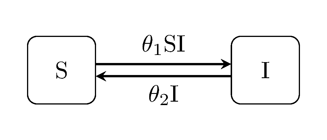
Individuals are assumed to take one of n discrete states –in this case Susceptible or Infectious.

Individuals are also assumed to 'migrate' back and forth between states, randomly, at rates defined as a function of the overall system state. For example here the rate of the new infections (S -> I) is defined by product of the number of infectious, and the number of susceptible individuals, scaled by an unknown contact rate parameter: $\beta$.

Bayesian inference

\[\pi(\theta|y) = \frac{\pi(\theta) \pi(y|\theta)}{\pi(y)} \propto \pi(\theta) \pi(y|\theta)\]

\[\begin{aligned} \theta := parameters \\ y := data \\ \pi(y|\theta) := f(\theta) \\ \pi(y) := model evidence \end{aligned}\]

Defining models

Predefined models

The package includes a set of predefined models, which can be instantiated easily:

import DiscretePOMP               # simulation / inference for epidemiological models
import Random               # other assorted packages used incidentally
import DataFrames
import Distributions

model = generate_model("SIS", [100,1])

Customising models

Models can also be specified manually. This is described further in the Models section.

Simulation

The main purpose of the package is to provide an automated framework for parameter inference, described in the next section. However much can also be learned from the use of simulated data; data obtained by generating [i.e. sampling] realisations of the model, generally referred to herein as 'trajectories'. For example, it can be an aid to intuition with respect to the internal dynamics mathematically described by the model, or as a method for predicting system behaviour under certain conditions.

The package implements the Gillespie direct method algorithm for simulation. It can be invoked thusly:

Random.seed!(1)
theta = [0.003, 0.1]
x = gillespie_sim(model, theta)	  # run simulation
p = plot_trajectory(x)            # plot (optional)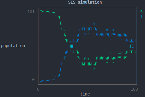

Inference

Here we demonstrate the package's functionality for [single-model] Bayesian inference using two of the algorithms implemented by the package; data-augmented Markov chain Monte Carlo (MCMC), and iterative-batch-importance sampling (IBIS).

First though, it is necessary to define an appropriate prior distribution, using the Distributions package:

model.prior = Distributions.Product(Distributions.Uniform.(zeros(2), [0.1, 0.5]))

MCMC

The first inference algorithm is MCMC; is a form of rejection sampling. The default number of Markov chains run for an analysis is three, and the Gelman-Rubin convergence diagnostic is carried out by default:

results = run_mcmc_analysis(model, y)
tabulate_results(results)
# trace plot of contact parameter (optional)
println(plot_parameter_trace(results, 1))

IBIS

The second class of algorithm we demonstrate here, is iterative-batch-importance sampling.

results = run_ibis_analysis(model, y)
tabulate_results(results)

The default configuration is particle [filter]-IBIS (i.e. the SMC^2 algorithm) but MBP can be used instead.

Model comparison

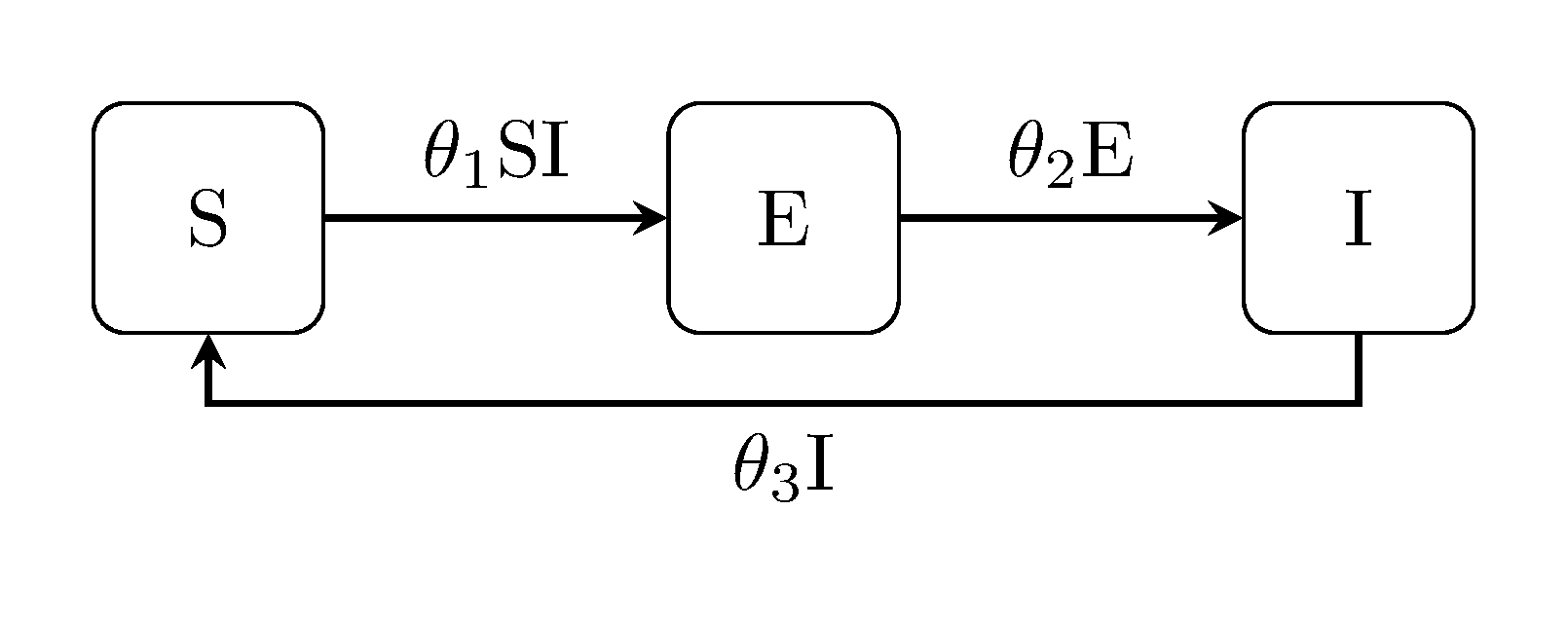
Finally, we describe how to compare models using the Bayes factor. First, we define an SEIS model to compare the SIS model/data with:

# define model to compare against
seis_model = generate_model("SEIS", [100,0,1])
seis_model.prior = Distributions.Product(Distributions.Uniform.(zeros(3), [0.1,0.5,0.5]))
seis_model.obs_model = partial_gaussian_obs_model(2.0, seq = 3, y_seq = 2)

seq here denotes the compartment that is observed (i.e. infectious individuals) in the SEIS model state space. Since the observations data y is formatted based on the SIS model, we also specify that column as y_seq.

Finally, we run the comparison, tabulate and plot the results:

# run comparison
models = [model, seis_model]
mcomp = run_model_comparison_analysis(models, y)
tabulate_results(mcomp; null_index = 1)
println(plot_model_comparison(mcomp))